公司动态

公

司

发

展

和

变

化

零基础人工智能-第二篇 TensorFlow2.0 手把手教程-玩转图像精准分类

2020-04-15

TF2.0与TF1.0区别

首先简单介绍下TF2.0与TF1.0区别。

数据集的切换

从tensorflow.examples.tutorials.mnist 切换到tensorflow.keras.datasets。

keras的接口成为了主力

datasets, layers, models都是从Keras引入的，而且在网络的搭建上，代码更少，更为简洁图形化界面更简便。

Fashion Mnist库，建立简单图像分类

接下来介绍图像分类操作基本流程，学习模型训练和分类的基本过程。

1. 下载matplotlib库

pip install -i https://pypi.tuna.tsinghua.edu.cn/simple matplotlib

2. 新建项目

打开jupyther notebook新建一个python3.0项目，导入库，同时查看使用的TF版本。

from __future__ import absolute_import, division, print_function

import tensorflow as tf

from tensorflow import keras

from tensorflow.keras import layers

import numpy as np

import matplotlib.pyplot as plt

print(tf.__version__)

TF版本为2.0。

3. 获取Fashion MNIST数据集

使用Fashion MNIST数据集，其中包含了10个类别中的70,000个灰度图像。图像显示了低分辨率（28 x 28像素）的单件服装。

Fashion MNIST旨在替代经典的MNIST数据集，通常用作计算机视觉机器学习计划的“Hello，World”。我们将使用60,000张图像来训练网络和10,000张图像，以评估网络学习图像分类的准确程度。

获取mnist数据集

(train_images,train_labels),(test_images, test_labels) = keras.datasets.fashion_mnist.load_data()

每个图像都映射到一个标签。由于类名不包含在数据集中，因此将它们存储在此处以便在绘制图像时使用：

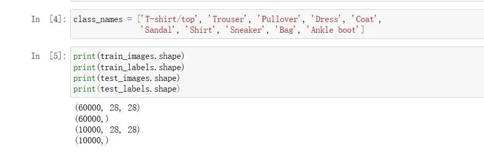
class_names = ['T-shirt/top', 'Trouser', 'Pullover', 'Dress', 'Coat',
'Sandal', 'Shirt', 'Sneaker', 'Bag', 'Ankle boot']

4. 探索数据

我们在训练模型之前探索数据集的格式。以下显示训练集中有60,000个图像，每个图像表示为28 x 28像素：

print(train_images.shape)

print(train_labels.shape)

print(test_images.shape)

print(test_labels.shape)

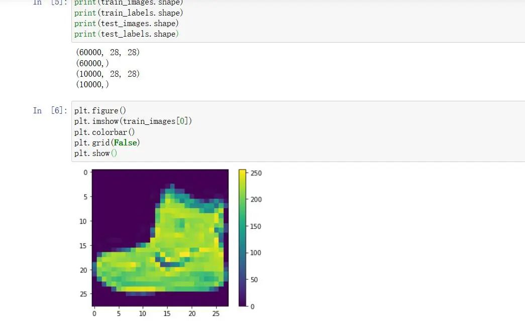
5. 处理数据

plt.figure()

plt.imshow(train_images[0])

plt.colorbar()

plt.grid(False) #

plt.show()

图片展示第一个图片鞋子

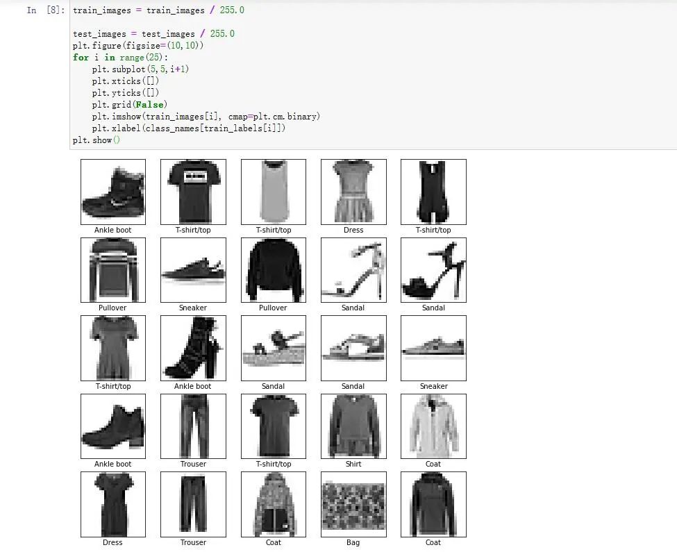
预处理和绘图

train_images = train_images / 255.0

test_images = test_images / 255.0

plt.figure(figsize=(10,10))

for i in range(25):

plt.subplot(5,5,i+1)

plt.xticks([])

plt.yticks([])

plt.grid(False)

plt.imshow(train_images[i], cmap=plt.cm.binary)

plt.xlabel(class_names[train_labels[i]])

plt.show()

除以255.0是为了图像值转到0到1之间的浮点型，除数是255.0浮点型，商值也为浮点型。然后将值送进神经网络模型内。这里训练集和测试机一样处理。

接下来是显示训练集前25张图片，包含类别名称，方便统计分类的类别。

6.构建网络

model = keras.Sequential(

[

layers.Flatten(input_shape=[28, 28]),

layers.Dense(128, activation='relu'),

layers.Dense(10, activation='softmax')

])

model.compile(optimizer='adam',

loss='sparse_categorical_crossentropy',

metrics=['accuracy'])

和上文测试用例类似。

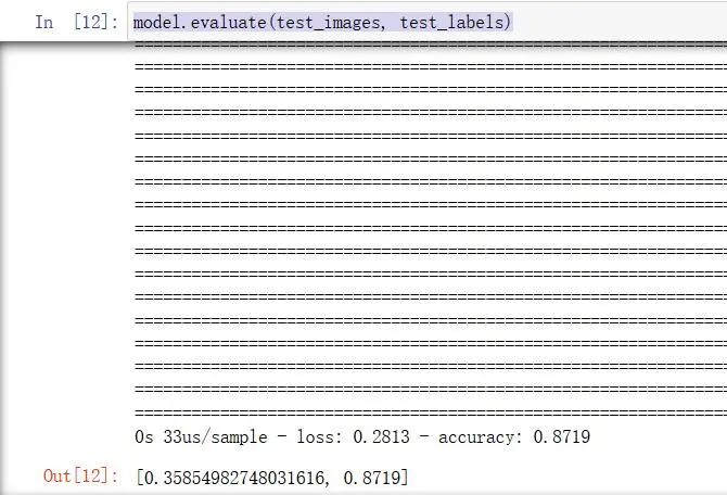
7. 训练与验证

训练分类：分类正确，准确率在80%左右。

model.fit(train_images, train_labels, epochs=5)

验证准确率：用了测试图集和标签，验证分类准确率。

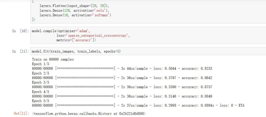
model.evaluate(test_images, test_labels)

8. 预测

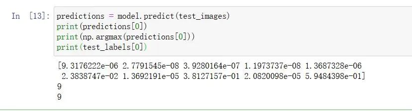
模型经过训练后，我们可以使用它对一些图像进行预测。

predictions = model.predict(test_images)

print(predictions[0])

print(np.argmax(predictions[0]))

print(test_labels[0])

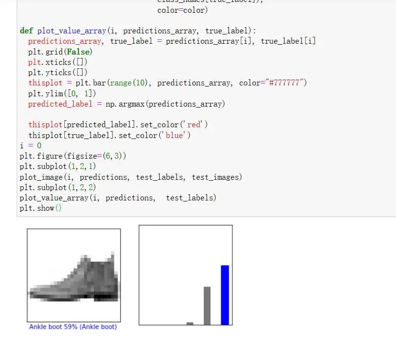
预测结果是一个具有 10 个数字的数组。这些数字说明模型对于图像对应于 10 种不同服饰中每一个服饰的“置信度”。我们可以看到哪个标签的置信度值最大（argmax）为9，靴子。

9. 绘制预测图

def plot_image(i, predictions_array, true_label, img):

predictions_array, true_label, img = predictions_array[i], true_label[i], img[i]

plt.grid(False)

plt.xticks([])

plt.yticks([])

plt.imshow(img, cmap=plt.cm.binary)

predicted_label = np.argmax(predictions_array)

if predicted_label == true_label:

color = 'blue'

else:

color = 'red'

plt.xlabel("{} {:2.0f}% ({})".format(class_names[predicted_label],

100*np.max(predictions_array),

class_names[true_label]),

color=color)

def plot_value_array(i, predictions_array, true_label):

predictions_array, true_label = predictions_array[i], true_label[i]

plt.grid(False)

plt.xticks([])

plt.yticks([])

thisplot = plt.bar(range(10), predictions_array, color="#777777")

plt.ylim([0, 1])

predicted_label = np.argmax(predictions_array)

thisplot[predicted_label].set_color('red')

thisplot[true_label].set_color('blue')

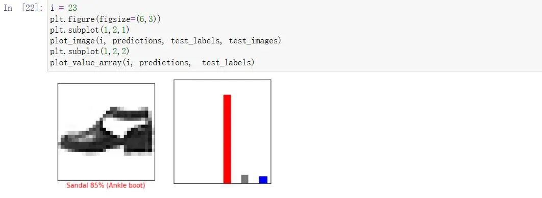
i = 0

plt.figure(figsize=(6,3))

plt.subplot(1,2,1)

plot_image(i, predictions, test_labels, test_images)

plt.subplot(1,2,2)

plot_value_array(i, predictions, test_labels)

plt.show()

蓝色预测正确概率是59%可信度。

i = 21

plt.figure(figsize=(6,3))

plt.subplot(1,2,1)

plot_image(i, predictions, test_labels, test_images)

plt.subplot(1,2,2)

plot_value_array(i, predictions, test_labels)

红色预测错误85%可信度是sandal凉鞋，但实际是靴子。

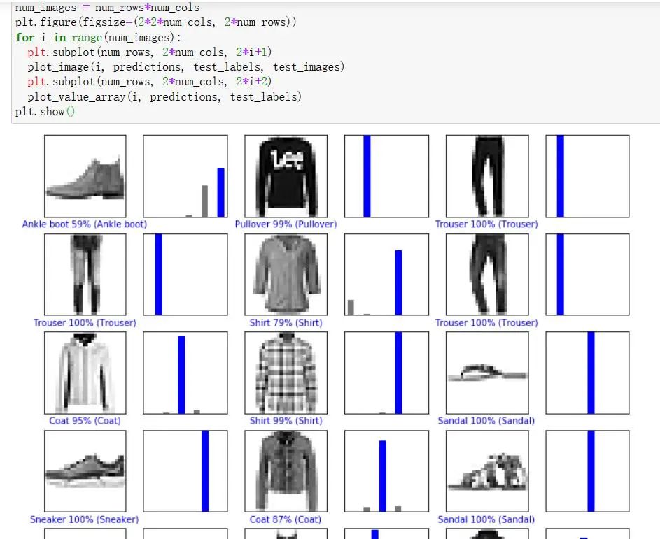
num_rows = 5

num_cols = 3

num_images = num_rows*num_cols

plt.figure(figsize=(2*2*num_cols, 2*num_rows))

for i in range(num_images):

plt.subplot(num_rows, 2*num_cols, 2*i+1)

plot_image(i, predictions, test_labels, test_images)

plt.subplot(num_rows, 2*num_cols, 2*i+2)

plot_value_array(i, predictions, test_labels)

plt.show()

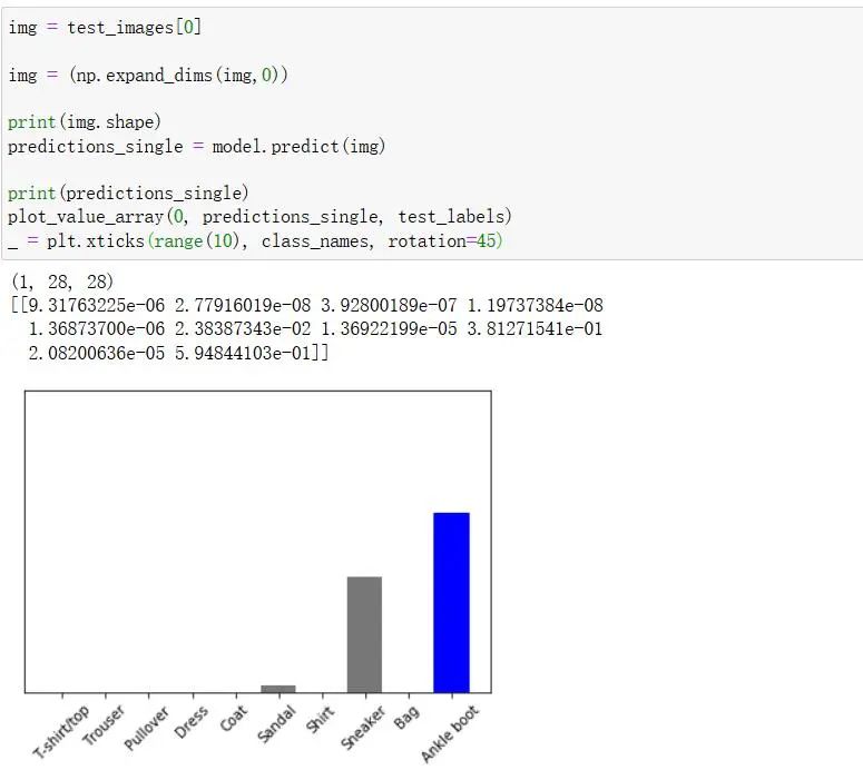
绘制统计预测图

或是单个图像预测，绘制单个图像预测值。

img = test_images[0]

img = (np.expand_dims(img,0))

print(img.shape)

predictions_single = model.predict(img)

print(predictions_single)

plot_value_array(0, predictions_single, test_labels)

_ = plt.xticks(range(10), class_names, rotation=45)